Introduction
TensorFlow is an incredibly powerful new framework for deep learning. The “MNIST For ML Beginners” and “Deep MNIST for Experts” TensorFlow tutorials give an excellent introduction to the framework. This article acts as a follow-on tutorial which addresses the following issues:
- The above tutorials use the MNIST dataset of hand written numbers, which pre-exists in TensorFlow TFRecord format and is loaded automatically. This can be a bit mysterious if you have no experience of data format manipulation in TensorFlow.
- Since the MNIST dataset is fixed, there is little scope for experimentation through adjusting the images and network to get a feel for how to deal with particular aspects of real data.
Here,
- You create your own images in a standard “png” format (that you can easily view), and you convert to TensorFlow TFRecord format. These are images of shapes created from python using the matplotlib module.
- You are free to explore by changing the way the images are created (contents, resolution, number of classes …).
The aim is to help you get to the point where you are comfortable in using TensorFlow with your own data, and also provide the opportunity for you to experiment by creating different datasets and adjusting the neural network accordingly. This tutorial assumes you are using a UNIX based system such as Linux or OSX.
Shape Sorting
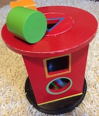
If you can’t find a toddler to sort your shapes for you, don’t worry: help is here. You are going to learn how to create a virtual shape sorting algorithm.
Creating the shapes
You will create images of shapes using the Matplotlib python module. If you don’t already have this on your system then please see the installation instructions here.
We are going to use python to create images of shapes with random positions and sizes: to keep things simple we are going to stick to 2 classes (squares and triangles), and to keep training time reasonable we are going to use low resolution of 32x32 (similar to the 28x28 of MNIST) - after the tutorial you can adjust these to your satisfaction.
First, create a new directory to work in:
mkdir shapesorter
cd shapesorter
Now set up some directories to contain training and validation data, for each of our two classes (squares and triangles)
mkdir -p data/train/squares
mkdir -p data/train/triangles
mkdir -p data/validate/squares
mkdir -p data/validate/triangles
The python script to automatically create a set of squares and triangles is below. This uses random numbers to vary position and size of these shapes. Please read through the comments in the script which describe the different stages.
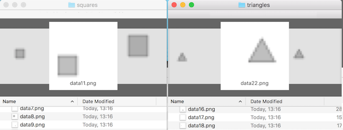
import matplotlib.path as mpath
import matplotlib.patches as mpatches
import matplotlib.pyplot as plt
import random
import math

#number of images we are going to create in each of the two classes
nfigs=4000

# Specify the size of the image.
# E.g. size=32 will create images with 32x32 pixels.
size=32

#loop over classes
for clss in ["squares","triangles"]:
    print "generating images of "+clss+":"

    #loop over number of images to generate
    for i in range(nfigs):

        #initialise a new figure
        fig, ax = plt.subplots()

        #initialise a new path to be used to draw on the figure
        Path = mpath.Path

        #set position and scale of each shape using random numbers
        #the coefficients are used to just try and prevent too many shapes from
        #spilling off the edge of the image
        basex=0.7*random.random()
        basey=0.7*random.random()
        length=0.5*random.random()

        if clss == "squares":
            path_data= [
                (Path.MOVETO, (basex, basey)), #move to base position of this image
                (Path.LINETO, (basex+length, basey)), #draw line across to the right
                (Path.LINETO, (basex+length, basey+length )), #draw line up
                (Path.LINETO, (basex, basey+length)), #draw line back across to the left
                (Path.LINETO, (basex, basey)), #draw line back down to base postiion
            ]
        else: #triangles
            path_data= [
                (Path.MOVETO, (basex, basey)), #move to base position of this image
                (Path.LINETO, (basex+length, basey)), #draw line across to the right
                (Path.LINETO, ((basex+length/2.),
                    basey+(math.sqrt(3.)*length/2.))), #draw line to top of equilateral triangle
                (Path.LINETO, (basex, basey)), #draw line back to base position
            ]

        #get the path data in the right format for plotting
        codes, verts = zip(*path_data)
        path = mpath.Path(verts, codes)

        #add shade the interior of the shape
        patch = mpatches.PathPatch(path, facecolor='gray', alpha=0.5)
        ax.add_patch(patch)

        #set the scale of the overlall plot
        plt.xlim([0,1])
        plt.ylim([0,1])

        #swith off plotting of the axis (only draw the shapes)
        plt.axis('off')

        #set the number of inches in each dimension to one
        # - we will control the number of pixels in the next command
        fig.set_size_inches(1, 1)

        # save the figure to file in te directory corresponding to its class
        # the dpi=size (dots per inch) part sets the overall number of pixels to the
        # desired value
        fig.savefig('data/train/'+clss+'/data'+str(i)+'.png',dpi=size)
        # close the figure
        plt.close(fig)
You now have a selection of 4000 squares and 4000 triangles in the train/squares and train/triangles directories respectively:
Now, we will move a quarter of these to the validate/squares and validate/triangles directories:
mv data/train/squares/data3*  data/validate/squares/.
mv data/train/triangles/data3*  data/validate/triangles/.
Converting to TensorFlow format
Change into the data directory:
cd data
Create a file called mylabels.txt and write to it the names of our classes:
squares
triangles
Now, to convert our images to TensorFlow TFRecord format, we are going to just use the build_image_data.py script that is bundled with the Inception TensorFlow model. Get this by clinking on the above link, and then File->Save in your browser.
We can just use this a “black box” to convert our data (but we get some insight as to what it is doing later when we read the data within TensorFlow). Run the following command
python build_image_data.py --train_directory=./train --output_directory=./  \
--validation_directory=./validate --labels_file=mylabels.txt   \
--train_shards=1 --validation_shards=1 --num_threads=1
We have told the script where to find the input files, and labels, and it will create a file containing all training images train-00000-of-00001 and another containing all validation images validation-00000-of-00001 in TensorFlow TFRecord format. We can now use these to train and validate our model.
Now change back up to the top-level directory:
cd ..
Training the model
In this section will see how to read in the previously generated TensorFlow TFRecord data files, and train the model. Please see the comments in each of the code snippets below. The full script can be downloaded here.
First, we import the required modules and set some parameters:
import tensorflow as tf
import sys
import numpy

#number of classes is 2 (squares and triangles)
nClass=2

#simple model (set to True) or convolutional neural network (set to False)
simpleModel=True

#dimensions of image (pixels)
height=32
width=32
Now, we can define a function which instructs TensorFlow how to read the data:
[UPDATE (17th March 2017): below script updated to be compatible with TensorFlow 1.X - "pack" replaced with "stack".]
# Function to tell TensorFlow how to read a single image from input file
def getImage(filename):
    # convert filenames to a queue for an input pipeline.
    filenameQ = tf.train.string_input_producer([filename],num_epochs=None)

    # object to read records
    recordReader = tf.TFRecordReader()

    # read the full set of features for a single example
    key, fullExample = recordReader.read(filenameQ)

    # parse the full example into its' component features.
    features = tf.parse_single_example(
        fullExample,
        features={
            'image/height': tf.FixedLenFeature([], tf.int64),
            'image/width': tf.FixedLenFeature([], tf.int64),
            'image/colorspace': tf.FixedLenFeature([], dtype=tf.string,default_value=''),
            'image/channels':  tf.FixedLenFeature([], tf.int64),
            'image/class/label': tf.FixedLenFeature([],tf.int64),
            'image/class/text': tf.FixedLenFeature([], dtype=tf.string,default_value=''),
            'image/format': tf.FixedLenFeature([], dtype=tf.string,default_value=''),
            'image/filename': tf.FixedLenFeature([], dtype=tf.string,default_value=''),
            'image/encoded': tf.FixedLenFeature([], dtype=tf.string, default_value='')
        })


    # now we are going to manipulate the label and image features

    label = features['image/class/label']
    image_buffer = features['image/encoded']

    # Decode the jpeg
    with tf.name_scope('decode_jpeg',[image_buffer], None):
        # decode
        image = tf.image.decode_jpeg(image_buffer, channels=3)

        # and convert to single precision data type
        image = tf.image.convert_image_dtype(image, dtype=tf.float32)


    # cast image into a single array, where each element corresponds to the greyscale
    # value of a single pixel.
    # the "1-.." part inverts the image, so that the background is black.

    image=tf.reshape(1-tf.image.rgb_to_grayscale(image),[height*width])

    # re-define label as a "one-hot" vector
    # it will be [0,1] or [1,0] here.
    # This approach can easily be extended to more classes.
    label=tf.stack(tf.one_hot(label-1, nClass))

    return label, image
# associate the "label" and "image" objects with the corresponding features read from
# a single example in the training data file
label, image = getImage("data/train-00000-of-00001")

# and similarly for the validation data
vlabel, vimage = getImage("data/validation-00000-of-00001")

# associate the "label_batch" and "image_batch" objects with a randomly selected batch---
# of labels and images respectively
imageBatch, labelBatch = tf.train.shuffle_batch(
    [image, label], batch_size=100,
    capacity=2000,
    min_after_dequeue=1000)

# and similarly for the validation data
vimageBatch, vlabelBatch = tf.train.shuffle_batch(
    [vimage, vlabel], batch_size=100,
    capacity=2000,
    min_after_dequeue=1000)

# interactive session allows inteleaving of building and running steps
sess = tf.InteractiveSession()

# x is the input array, which will contain the data from an image
# this creates a placeholder for x, to be populated later
x = tf.placeholder(tf.float32, [None, width*height])
# similarly, we have a placeholder for true outputs (obtained from labels)
y_ = tf.placeholder(tf.float32, [None, nClass])
tf.train.shuffle_batch function is being used to get a randomly selected batch of 100 images from the data set. The other parameters in this function call can be adjusted for performance as described [here](https://www.tensorflow.org/versions/r0.11/api_docs/python/io_ops.html#shuffle_batch).
We are now ready to define the model. First, the simple model (adapted from "MNIST For ML Beginners"):
if simpleModel:
  # run simple model y=Wx+b given in TensorFlow "MNIST" tutorial

  print "Running Simple Model y=Wx+b"

  # initialise weights and biases to zero
  # W maps input to output so is of size: (number of pixels) * (Number of Classes)
  W = tf.Variable(tf.zeros([width*height, nClass]))
  # b is vector which has a size corresponding to number of classes
  b = tf.Variable(tf.zeros([nClass]))

  # define output calc (for each class) y = softmax(Wx+b)
  # softmax gives probability distribution across all classes
  y = tf.nn.softmax(tf.matmul(x, W) + b)
else:
  # run convolutional neural network model given in "Expert MNIST" TensorFlow tutorial

  # functions to init small positive weights and biases
  def weight_variable(shape):
    initial = tf.truncated_normal(shape, stddev=0.1)
    return tf.Variable(initial)

  def bias_variable(shape):
    initial = tf.constant(0.1, shape=shape)
    return tf.Variable(initial)

  # set up "vanilla" versions of convolution and pooling
  def conv2d(x, W):
    return tf.nn.conv2d(x, W, strides=[1, 1, 1, 1], padding='SAME')

  def max_pool_2x2(x):
    return tf.nn.max_pool(x, ksize=[1, 2, 2, 1],
                          strides=[1, 2, 2, 1], padding='SAME')

  print "Running Convolutional Neural Network Model"
  nFeatures1=32
  nFeatures2=64
  nNeuronsfc=1024

  # use functions to init weights and biases
  # nFeatures1 features for each patch of size 5x5
  # SAME weights used for all patches
  # 1 input channel
  W_conv1 = weight_variable([5, 5, 1, nFeatures1])
  b_conv1 = bias_variable([nFeatures1])

  # reshape raw image data to 4D tensor. 2nd and 3rd indexes are W,H, fourth
  # means 1 colour channel per pixel
  # x_image = tf.reshape(x, [-1,28,28,1])
  x_image = tf.reshape(x, [-1,width,height,1])


  # hidden layer 1
  # pool(convolution(Wx)+b)
  # pool reduces each dim by factor of 2.
  h_conv1 = tf.nn.relu(conv2d(x_image, W_conv1) + b_conv1)
  h_pool1 = max_pool_2x2(h_conv1)

  # similarly for second layer, with nFeatures2 features per 5x5 patch
  # input is nFeatures1 (number of features output from previous layer)
  W_conv2 = weight_variable([5, 5, nFeatures1, nFeatures2])
  b_conv2 = bias_variable([nFeatures2])


  h_conv2 = tf.nn.relu(conv2d(h_pool1, W_conv2) + b_conv2)
  h_pool2 = max_pool_2x2(h_conv2)


  # denseley connected layer. Similar to above, but operating
  # on entire image (rather than patch) which has been reduced by a factor of 4
  # in each dimension
  # so use large number of neurons

  # check our dimensions are a multiple of 4
  if (width%4 or height%4):
    print "Error: width and height must be a multiple of 4"
    sys.exit(1)

  W_fc1 = weight_variable([(width/4) * (height/4) * nFeatures2, nNeuronsfc])
  b_fc1 = bias_variable([nNeuronsfc])

  # flatten output from previous layer
  h_pool2_flat = tf.reshape(h_pool2, [-1, (width/4) * (height/4) * nFeatures2])
  h_fc1 = tf.nn.relu(tf.matmul(h_pool2_flat, W_fc1) + b_fc1)

  # reduce overfitting by applying dropout
  # each neuron is kept with probability keep_prob
  keep_prob = tf.placeholder(tf.float32)
  h_fc1_drop = tf.nn.dropout(h_fc1, keep_prob)

  # create readout layer which outputs to nClass categories
  W_fc2 = weight_variable([nNeuronsfc, nClass])
  b_fc2 = bias_variable([nClass])

  # define output calc (for each class) y = softmax(Wx+b)
  # softmax gives probability distribution across all classes
  # this is not run until later
  y=tf.nn.softmax(tf.matmul(h_fc1_drop, W_fc2) + b_fc2)
# measure of error of our model
# this needs to be minimised by adjusting W and b
cross_entropy = tf.reduce_mean(-tf.reduce_sum(y_ * tf.log(y), reduction_indices=[1]))

# define training step which minimises cross entropy
train_step = tf.train.AdamOptimizer(1e-4).minimize(cross_entropy)

# argmax gives index of highest entry in vector (1st axis of 1D tensor)
correct_prediction = tf.equal(tf.argmax(y,1), tf.argmax(y_,1))

# get mean of all entries in correct prediction, the higher the better
accuracy = tf.reduce_mean(tf.cast(correct_prediction, tf.float32))
[UPDATE (17th March 2017): below script updated to be compatible with TensorFlow 1.X - "initialize_all_variables" replaced with "global_variables_initializer".]
# initialize the variables
sess.run(tf.global_variables_initializer())

# start the threads used for reading files
coord = tf.train.Coordinator()
threads = tf.train.start_queue_runners(sess=sess,coord=coord)

# start training
nSteps=1000
for i in range(nSteps):

    batch_xs, batch_ys = sess.run([imageBatch, labelBatch])

    # run the training step with feed of images
    if simpleModel:
      train_step.run(feed_dict={x: batch_xs, y_: batch_ys})
    else:
      train_step.run(feed_dict={x: batch_xs, y_: batch_ys, keep_prob: 0.5})


    if (i+1)%100 == 0: # then perform validation

      # get a validation batch
      vbatch_xs, vbatch_ys = sess.run([vimageBatch, vlabelBatch])
      if simpleModel:
        train_accuracy = accuracy.eval(feed_dict={
          x:vbatch_xs, y_: vbatch_ys})
      else:
        train_accuracy = accuracy.eval(feed_dict={
          x:vbatch_xs, y_: vbatch_ys, keep_prob: 1.0})
      print("step %d, training accuracy %g"%(i+1, train_accuracy))


# finalise
coord.request_stop()
coord.join(threads)
simpleModel=Trueto
simpleModel=Falseto run the convolutional neural network (from "Deep MNIST for Experts") and run again: you will see the accuracy increase to between 95% and 100%.
Further Work
Image Resolution
Increase the resolution of the images you create to, say, 128x128 pixels, and train using these larger images (remembering to set the size properly at the top of the training script). You should see similar behaviour (but the training time will be longer).Importance of Validation Set
See what happens when you train using squares for both classes. As expected, the accuracy should be around 50% (i.e. the ability to predict is no better a uneducated guess since there is no conceptual difference between the classes). Now, temporarily replace the linevbatch_xs, vbatch_ys = sess.run([vimageBatch, vlabelBatch])with
vbatch_xs, vbatch_ys = sess.run([imageBatch, labelBatch])to use the training images themselves for validation. You will see that this is a bad idea since the accuracy rises significantly above 50%, which is misleading. This demonstrating the importance of using a separate set of images for validation of the model.